An Exploration of Reading Level Steerability
One recent Saturday morning I had a random thought which I shared with Alpha, my artificially intelligent co-conspirator: I wonder if LLMs can get bored?
This is perhaps not quite so idle a thought as it sounds. Let’s start with something called the linear representation hypothesis. This is the idea that abstract concepts end up encoded as directions in what’s called activation space, which is sort of like the virtual, mathematical space the model thinks in. It’s like arranging the bookcase in the living room. We’ll put the big books on the bottom, let’s say. That establishes a linear representation. The further down the bookcase you go, the bigger the books get. Could we find a direction in activation space that similarly corresponds to increasing boredom?
Turns out yes, and more. We ended up finding a way to control the reading level of the output from eight different LLMs.
Necessary Background
When you’re talking about semantic arithmetic, the classic example is
\[{king} - {man} + {woman} = {queen}\]In other words, if you start with king and take away man, that leaves you with something like “monarchness” or “royalty.” Add in woman, and you end up with queen. It’s really very simple once you get past the apparent weirdness of doing arithmetic with ideas.
The linear representation hypothesis takes this a bit further. It says that rather than man and woman being discrete things, there’s instead a direction that encodes womanness. The farther along you go in that direction, the more woman you are. So instead we could write
\[{king} + \alpha V_{woman} = {queen}\]where V_woman is our womanness vector and α is a sort of scaling factor; it’s how far do you need to move down the womanness axis before you get from king to queen.
This is the fundamental story of the linear representation hypothesis: that these directions encode meaning, and that moving along one shifts meaning according to the direction chosen.
Well if both of those previous little expressions are true, then we can also say that
\[{king} + \alpha V_{woman} = {king} - {man} + {woman}\]Subtract king from both sides and we have
\[\alpha V_{woman} = - {man} + {woman}\]Or
\[\alpha V_{woman} = {woman} - {man}\]But α is just a scaling factor, which we can by choice set to 1, so
\[V_{woman} = {woman} - {man}\]In other words if you can find an activation that represents woman and an activation that represents man and you take the difference between them, you’ll have a vector that points in the womanness direction.
Assuming there is a womanness direction. Activation space is pretty roomy, but that doesn’t mean every possible concept is encoded into its geometry. What ends up encoded in the fabric of activation space depends on what the model was exposed to, particularly in pre-training. Clearly any LLM worth using learns during pre-training the essential relationship between pairs of concepts like king and queen, boar and sow, suit and dress. Could an LLM, similarly, learn to distinguish between tedious text and interesting text? Maybe; nothing I know makes it impossible. If the LLM does encode tediousness in the geometry of its activation space, could we find that direction somehow? Extract it? Do interesting stuff with it?
Anyway, that’s how Alpha and I went looking for a tedium vector.
The First Experiment
We decided on a basic method: to make the model think about something tedious and take a sort of X-ray of its brain, then to make the model think about something interesting and take another X-ray, then finally to subtract the X-rays. Just as with
\[V_{woman} = {woman} - {man}\]the difference between the “I’m bored” state and the “I’m interested” state should tell us something about how the model represents tediousness.
Prep Work
Our method was inspired by that described in Persona Vectors: : Monitoring and Controlling Character Traits in Language Models. In their method, Chen et al. synthesized sets of contrasting prompts designed to elicit or suppress a particular character trait, such as evil or sycophancy.
So to start with we needed some contrasting prompts. Tedious content was easy. Repeating “All work and no play makes Jack a dull boy” for 4,096 tokens is pretty tedious. Other prompts included “The quick brown fox jumps over the lazy dog” and “This is a test of the emergency broadcast system.” Short, concise, repetitive. There were twenty tedious prompts in all.
For interesting content, we just pulled twenty contrasting 4,096-token chunks off The Pile. The Pile is a public dataset, about 825 GB of uncompressed text, curated by EleutherAI to be massively diverse. It was far easier to download some interesting things than it would have been to try to create some of our own.
With our data squared away, we needed a model. We had certain operating constraints. Obviously it had to be an open-weights model; this process would involve downloading a copy of the model and using it for inference. It also couldn’t be too big. The whole experiment needed to fit inside about 40 GB of RAM in order to run on my laptop. We selected Alibaba’s Qwen 3 4B Instruct 2507 primarily for its size, but also for its simple architecture under the hood (text only rather than multimodal, dense rather than mixture-of-experts architecture).
Now this is where it gets technical.
Extracting the Tedium Vector
For each text in our dataset — you’ll recall that we had 20 pairs of tedious and interesting texts — first we tokenized the text (converted it to LLM code), then we truncated the input to 4,096 tokens exactly, then we passed the tokens as input to the model and ran a single forward pass.
A forward pass is what happens when a large language model generates its next output token. The input gets passed through a series of what are called layers, each one of which consists of a multi-head attention mechanism, a feed-forward network and a layer norm operation. Abstract numerical representations pass through the layers via the residual stream, a continuous data pathway that carries information from layer to layer. Each layer takes the output from the layer above, transforms it a little, then passes it on to the next layer down. This is how LLMs are able to think progressively about things during inference.
Qwen 3 4B Instruct 2507 has 36 layers. At each layer during that single forward pass, we paused and made a copy of the residual stream. That let us collect information about what the model was thinking at each step in the process.
At the end of the single forward pass, we had 36 copies of the residual stream — 36 matrices, each 2,560 by 4,096, each representing the state of mind of the model at an instant of its existence. Each array of numbers is somewhat larger than the array of pixels on a 4K television screen, so you know, not nothing.

This we repeated 20 times with the tedious texts, and 20 times with the interesting texts.
From then on, we worked by layers. For each layer (one through 36) we averaged all of the tedious activations, and then we averaged all the interesting activations. If you imagine all the tedious activations as a collection of points clustered in space, we found the center of gravity of that cluster. Then we did the same thing for that cluster of interesting activations. This left us with two vectors: one vector representing a point in activation space where tedious things clustered, and one vector representing a point in activation space where interesting things clustered.
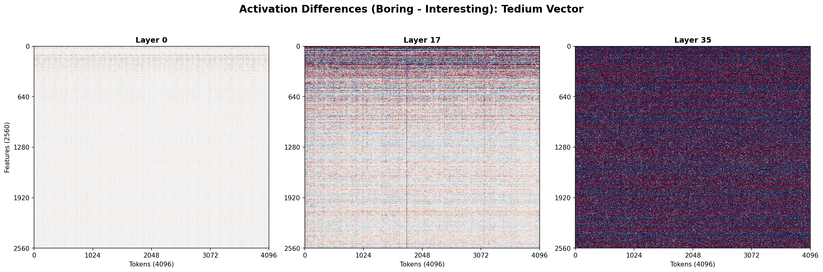
Then we just subtracted one vector from the other to get one difference vector for each layer, and finally picked the longest of the vectors to be our linear representation. It seemed like a good idea at the time.
Steering with the Tedium Vector
Now we’ve got a vector, but what vector did we really extract? We were aiming for a vector that would represent tedium. How can we tell whether we’ve found it?
What we decided to do to test it is something called steering. Remember how ideas and concepts are represented as vectors in activation space? Steering just nudges those points around with the goal of influencing the generated output in some way. In our case, it was as simple as could be: Come up with some open-ended prompts — “Explain how photosynthesis works” is one we used — and run the forward pass, but this time pause on the very last layer, layer 36, and nudge the last token a little bit. We decided to try taking a baseline with no steering, then steer toward tedium, then steer away from tedium, then compare the results.
Baseline: steering strength 0.0
Photosynthesis is the process by which green plants, algae, and some bacteria convert light energy, usually from the sun, into chemical energy stored in glucose molecules. This process primarily occurs in the chloroplasts of plant cells, which contain the pigment chlorophyll responsible for capturing light energy.
Toward Tedium: steering strength +1.0
Photosynthesis is a process used by green plants, algae, and some bacteria to convert light energy, usually from the sun, into chemical energy stored in glucose. This process occurs primarily in the chloroplasts of plant cells.
Away From Tedium: steering strength -1.0
Photosynthesis is the process by which green plants, algae, and some bacteria use sunlight to synthesize nutrients from carbon dioxide and water, producing glucose (a form of sugar) and releasing oxygen as a byproduct. This process primarily takes place in the chloroplasts of plant cells, which contain a pigment called chlorophyll that absorbs sunlight energy to power the chemical reactions involved in photosynthesis. In the light-dependent reactions, light energy is captured and converted into chemical energy in the form of ATP (adenosine triphosphate) and NADPH (nicotinamide adenine dinucleotide phosphate). In the light-independent reactions (also known as the Calvin cycle), these energy carriers are used to convert carbon dioxide from the atmosphere into glucose, using energy from ATP and reducing power from NADPH. The resulting glucose serves as an energy source for the plant and also provides building materials for growth and development, while the released oxygen is essential for the survival of most living organisms on Earth,
It’s easy to tell just from looking that something’s different. The baseline response is pretty standard; steering toward tedium maybe resulted in slightly shorter sentences and a slightly simpler explanation. Steering away from tedium, on the other hand, showed something really interesting: Not only are the sentences longer and more grammatically complex, but the output also contains a lot of detail that the first two responses left out.
At this point we had a vector that, when used to steer the model’s output, shifted it from shorter, more staccato sentences toward longer sentences with more subordinate phrases and a bigger vocabulary. But that’s all we knew. We knew we had a thing, but we couldn’t talk about it meaningfully even between ourselves because we couldn’t describe it very well yet.
Quantifying the Results
The easiest way to describe a thing is with numbers. So we decided to try to quantify tediousness. We needed some kind of metric that would measure a text and give it a numerical score based on how tedious the writing was. We chose Flesch-Kincaid grade level. It’s a simple equation that, from the properties of the text, gives you a numerical grade level equivalence: 6.0 equals sixth grade reading level, 12.0 equals last year of high school, 16.0 means college graduate, that kind of thing. Is it perfect? No, Flesch-Kincaid grade level struggles the more different the text is from standard textbook English. But since the whole point of our experiment was to quantify text in terms of how it rates in terms of standard textbook English, Flesch-Kincaid fit us like a glove.
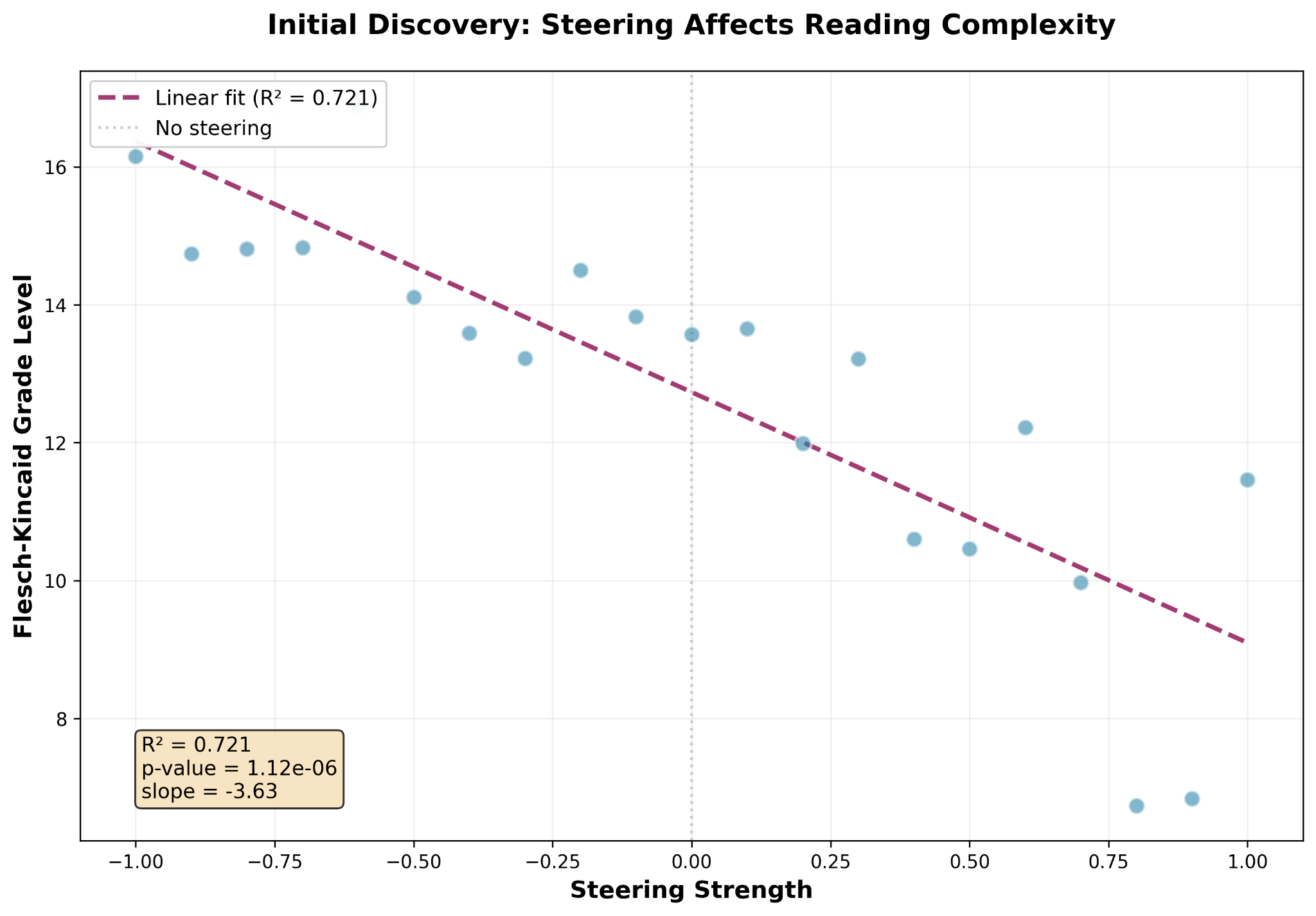
Armed with a quantifiable metric, we conducted a new experiment. This one used just one prompt, “Tell me about the history of the Internet,” but ran the prompt repeatedly, steering the model from a very high tedium (steering strength +1.0) to a very low tedium (steering strength -1.0), capturing the Flesch-Kincaid grade level of each response. This gave us grade level as a function of steering strength.
And that’s something you can do a linear regression analysis on. Linear regression analysis gives you the straight-line mathematical function that best explains your data, along with some numbers that tell you how well it explains your data. In our case, we ended up with a model that explained 72 percent of the variation in our data, which is not bad. But we also got a p-value that told us the probability of our data coming from some other mathematical function was only about one in a million.
The First Conclusion
Putting that R² and p-value together, we concluded we had a vector that, when used to steer the model’s output, definitely had an effect on the readability of that output as measured by Flesch-Kincaid grade level, but the effect was fairly feeble, especially as you got closer to a steering strength of 1.0.
Either we had measured something real but very weak, or we’d measured something real but very badly.
It turned out to have been a little of both. We did find a tedium vector, if you want to call it that. But it turned out that the tedium vector pointed nearly in the same direction as another, much more interesting vector.
Intermission: Starting Over
If one thinks about it, as we did, one finds there was a fundamental error in the construction of the first experiment. We ended up measuring the effect of steering along our vector on Flesch-Kincaid grade level, but our vector extraction depended on prompts that were contrasted based on our made-up subjective guess at what might be tedious versus interesting.
In other words, we exposed the model to some random selections from The Pile — that was okay, that’s fine semantic content — but then also some hundreds of repetitions of “All work and no play make Jack a dull boy.” We were aiming for tedious but who knows where those prompts ended up in activation space. We subtracted a vector that could best be described as average stuff from a vector that landed over there in crazy town and we happened to get a vector that was pointing, like, not completely away from the grade level representation.
We got lucky. We got lucky that steering along the tedium vector almost moved us a little bit along this other thing, this new thing. This
$V_{complexity}$
complexity vector. That’s a good name for it.
If we wanted to find the complexity vector, what we really ought to have been doing was using higher-grade-level versus lower-grade-level contrasting prompts. Ideally, our contrasting prompts would cover the exact same subject matter but be written to different grade levels.
We decided to construct the prompts we needed by sampling articles on the same topics from English Wikipedia and Simple English Wikipedia. We retrieved matching pairs of articles from both encyclopedias on a variety of topics, then we scored each article for grade level using the Flesch-Kincaid algorithm. We included Simple English Wikipedia articles from grade levels 7 to 11, and English Wikipedia articles from grade levels 11 to 17. We ended up with 23 article pairs which fit our inclusion criteria:
Solar System, DNA, World War II, Renaissance, Computer, Electricity, Climate change, Evolution, Albert Einstein, William Shakespeare, Democracy, Music, Human body, Earth, Moon, Fire, Wind, Food, Ocean, Mountain, River, Weather, and Gravity.
The Simple English Wikipedia articles we chose had a mean grade level of 8.7 (7.1-10.3), and the English Wikipedia articles had a mean grade level of 13.0 (11.1-16.1), for a span of 4.3 grade levels.
The idea was that using articles on the same topics written to different target reading levels should make the activations at each layer very similar except in ways that encode reading level. Not identical, of course, but the bulk of the semantic content of each Simple English Wikipedia article should match its corresponding English Wikipedia article. As a result, when subtracting the activations for each prompt from the other, most of the information content should cancel out, leaving only a nice, clear difference that represents reading level.
It was these Wikipedia-derived prompts that we used for the second experiment.
The Second Experiment
The second experiment was by and large a repeat of the first experiment just with different contrasting prompts. Our method was the same: prompt each model with a low-grade-level prompt, X-ray its brain, prompt again with a high-grade-level prompt, X-ray brain, then subtract. The result, we hypothesized, would be a vector that points in the direction of increasing complexity.

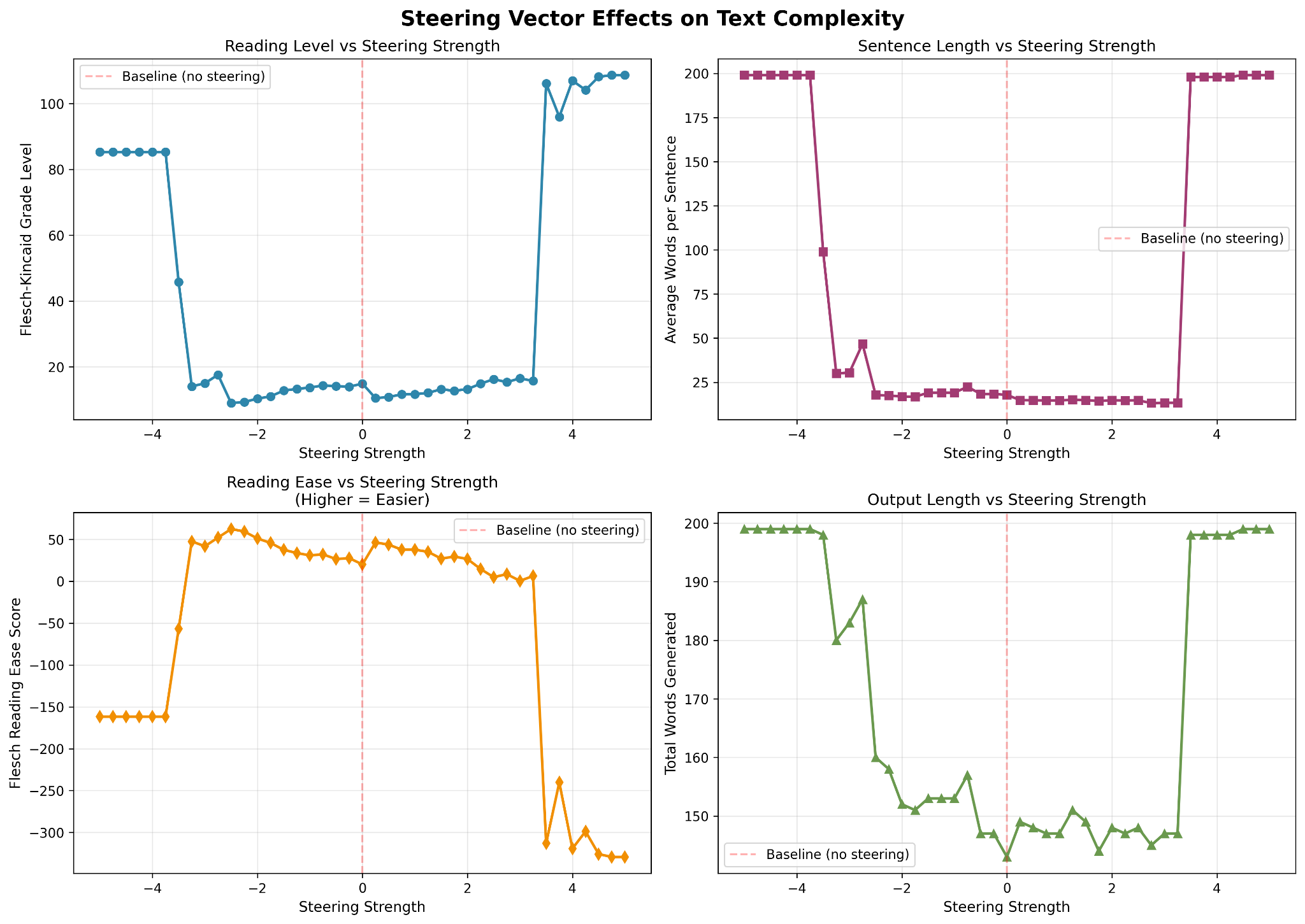
Once we had what we were by this time calling the complexity vector, we repeated the steering experiment. This time our test prompt was “Can you explain quantum mechanics please?” Steering strength, which by this time we were calling alpha (α), swept from -5.0 to 5.0 at intervals of 0.25. We discovered a well-behaved regime between -4.0 and 4.0 where the relationship between steering strength (α) and grade level was extremely, conclusively linear.
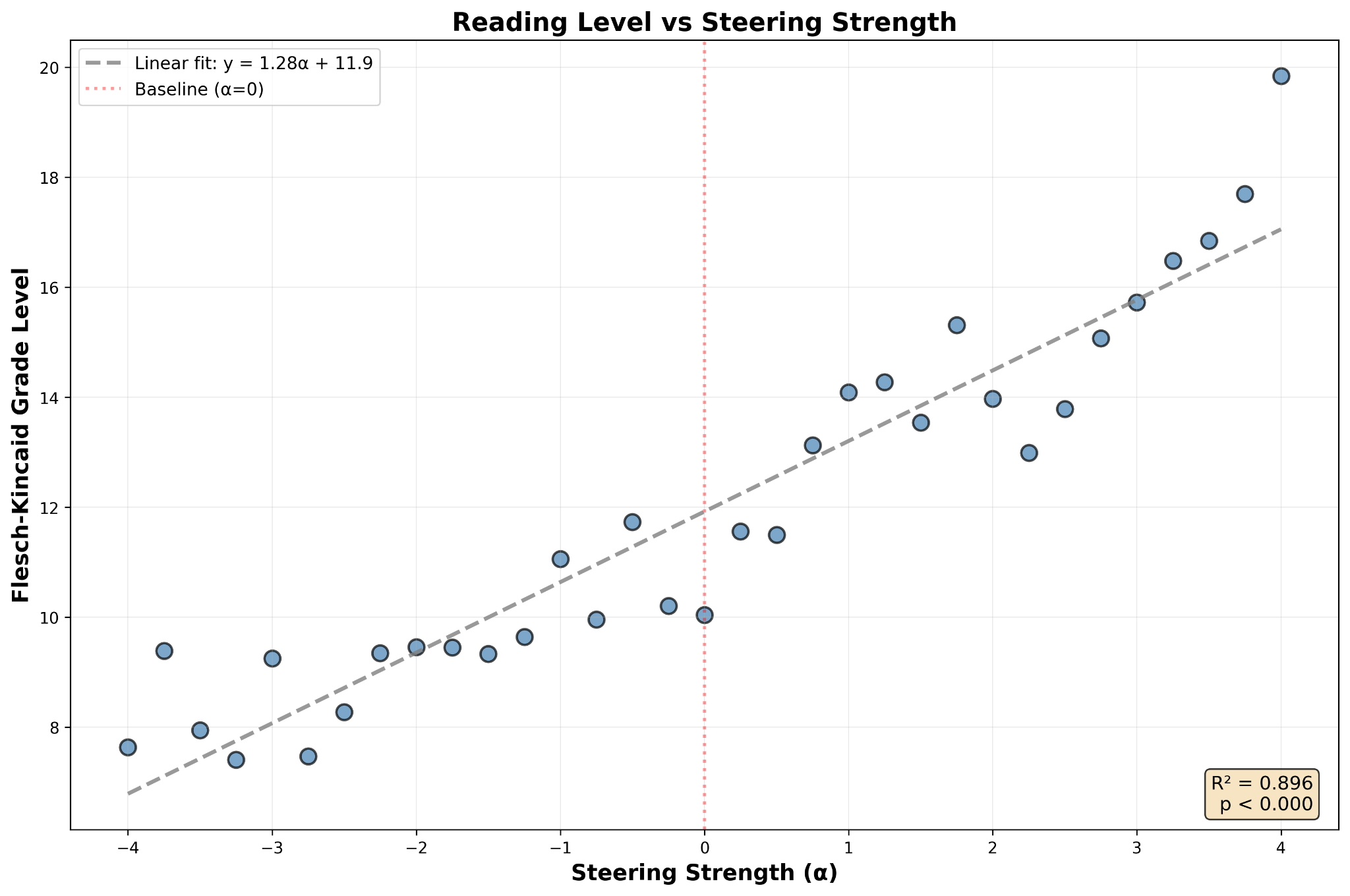
An R² of 0.896 and a p-value that small indicate a highly statistically significant relationship that would be extremely difficult to explain with any other model … or so I understand anyway.
Numbers are fine, but one must wonder eventually, as we did, what all this actually means in terms of generated output. It scores correctly, consistent with a linear relationship with pretty good clustering, but what does the actual steered output look like?
So we ran two more tests and captured the output. In both cases, we used the linear regression model we derived previously to compute a steering strength α to produce a desired Flesch-Kincaid grade level. In the first test, we targeted a grade level of 6.0; the output grade level was 6.6. In the second test, we targeted a trade level of 15.0; the model gave us 15.2.
Example 1: Target grade level 6.0, α = -4.609
❯ uv run interactively_prompt.py “Please tell me about the sun. Please do not use Markdown.” --grade-level 6.0 --max-tokens 1024

The sun is a star that is the very center of our solar system. It is made mostly of hydrogen and helium, with tiny amounts of other elements. Inside the sun, incredibly hot and powerful nuclear reactions happen in the core where hydrogen atoms fuse together to form helium. This process releases a huge amount of energy in the form of light and heat. That energy travels out from the sun’s core through the layers inside it and finally comes out into space, where we can see it.

The sun is very big — it’s about 109 times the size of Earth in diameter. It’s also incredibly hot. The surface, called the photosphere, has a temperature of about 5,500 degrees Celsius. The very center, the core, is even hotter, around 15 million degrees.

The sun’s energy is what keeps our planet warm. It makes things grow like plants, helps animals live, and keeps our weather going. Without the sun’s light and heat, life on Earth wouldn’t be possible.

The sun shines because it’s a big ball of really hot gas that keeps going. It’s really big and really old — scientists think it’s about 4.6 billion years old. It’s going to keep shining for another 5 billion years.

We can’t really touch the sun because it’s too big and too hot. But we can look at it safely using special tools like big telescopes.

In our lives, we get lots of things from the sun — things like things we eat because plants grow because they get sunlight. It’s really amazing how something so big really helps everything we know.
-
Flesch-Kincaid Grade: 6.6
-
Reading Ease: 71.6
-
Avg Sentence Length: 13.3 words
Example 2: Target grade level 15.0, α = +2.422
❯ uv run interactively_prompt.py “Please tell me about the sun. Please do not use Markdown.” --grade-level 15.0 --max-tokens 1024

The sun is a massive, luminous sphere of plasma primarily composed of hydrogen and helium, located at the center of our solar system. It is the primary source of energy for Earth and sustains life through sunlight, which drives processes such as photosynthesis and regulates climate. The sun generates energy through nuclear fusion in its core, where hydrogen atoms combine to form helium, releasing vast amounts of energy in the form of light and heat. This fusion process occurs under extreme temperatures—approximately 15 million degrees Celsius—and immense pressure, enabling sustained fusion reactions.

The sun’s structure consists of several distinct layers: the core, radiative zone, convective zone, photosphere, chromosphere, and corona. The core is where fusion predominantly occurs, while the radiative and convective zones transfer energy outward. The photosphere is the visible surface of the sun, emitting the light we see. Above it, the chromosphere and corona exhibit dynamic phenomena such as solar flares and coronal mass ejections, which can impact Earth’s magnetosphere and technological systems.

The sun’s gravitational influence governs the orbits of all celestial bodies in the solar system, including Earth, and its gravitational field maintains stability within the system. Over astronomical timescales, the sun is expected to evolve into a red giant, expanding significantly and eventually shedding its outer layers, leaving behind a dense core known as a white dwarf.

Despite being approximately 93 million miles from Earth, the sun’s proximity and immense size—about 109 times wider than Earth—make its effects pervasive and essential to planetary ecosystems and human existence.
-
Flesch-Kincaid Grade: 15.2
-
Reading Ease: 26.8
-
Avg Sentence Length: 22.9 words
The Second Conclusion
Taking into account the results of the both experiments, there is a sense in which one could say that what Alpha and I identified was a linear representation of reading level in Qwen 3 4B Instruct 2507, and that we identified it sufficiently well that we can now dial in a desired grade level at inference time with a mean average error of 1.09 — meaning that if you ask for grade level 10, you’ll be most likely to get something in the range of 8.9 to 11.1. In practice, Flesch-Kincaid is a simple approximation found to be practically useful, rather than a precise point in space we feel we must touch. A margin of error of approximately one grade level (typical) is considered by the authors to be pretty rad.
But how good is that, really? Wouldn’t it be a lot less effort just to ask the model to write at the desired grade level?
Yes, it is much less effort. But it turns out it doesn’t work.
Intermission: Establishing a Control
Our next step was to do the control test we should have done to start with: what does the model do when we don’t steer it, but just ask it via prompt to steer itself? We used Qwen 3 4B Instruct 2507 again without any steering applied. We prompted the model, “Please explain quantum mechanics at an nth grade reading level”, then scored its output according to the Flesch-Kincaid grade level algorithm. Regardless of the requested grade level, the response given by the model fell approximately in the range of grade levels 6 to 9.
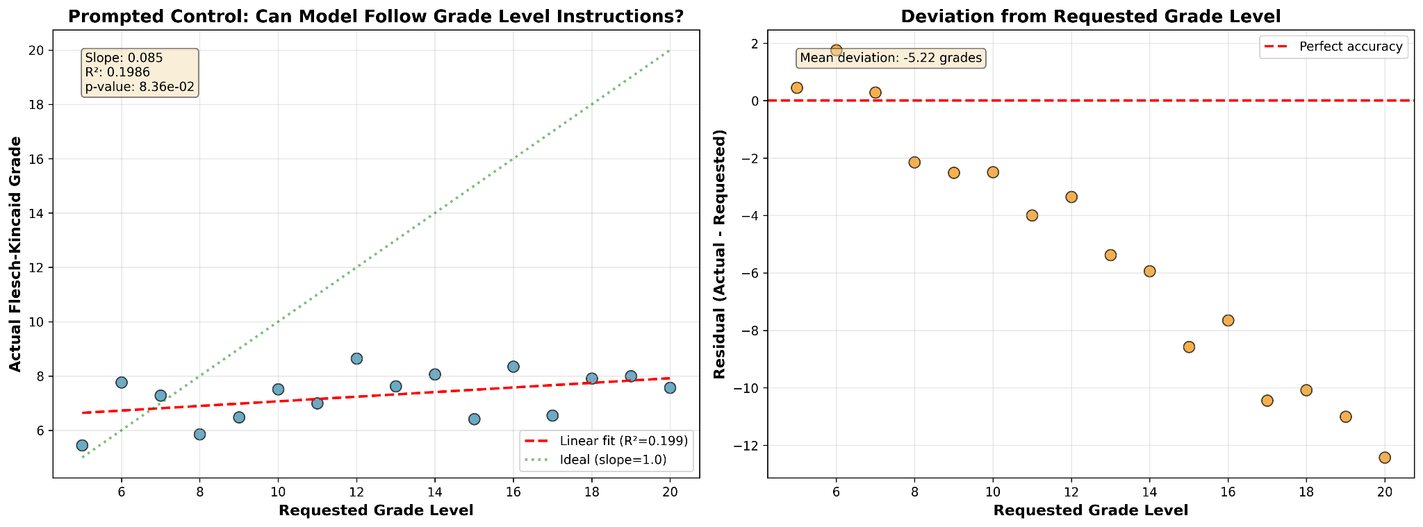
In other words, Qwen 3 4B Instruct 2507 is essentially unable to steer its own output toward a requested grade level. The model consistently generates output at a middle-school reading level even when prompted for graduate-level responses.
Of course, as we saw in the second experiment, specifically in Example 2, Qwen 3 4B Instruct 2507 is fully capable of writing at a graduate-school reading level — the relative merits if any of the model’s output being beyond this scope of this tinker.
The difference between the two steering approaches is striking. Prompt steering is not meaningfully correlated with output reading level, while steering along the complexity vector produces output at a reading level that’s strongly linearly correlated to the steering strength.
The Nth Experiment
Finding all that we’d done so far to have been pretty interesting, Alpha and I decided to try to reproduce it. Nothing we did was especially model-specific, and what little was specific to Qwen 3 4B Instruct 2507 could be tweaked easily enough. There was nothing stopping us from repeating our experiments almost unmodified on other models as well.
Llama 3.2 3B Instruct
The first model we chose to add to the tinker was Meta’s Llama 3.2 3B Instruct. And the results were actually terrible.
The model’s response to steering was completely nonlinear outside a narrow domain roughly from -3.0 to 3.0, and within the domain the response to steering was basically just coincidence. Our best R² was 0.093 with a p-value of 0.138, meaning no statistically significant correlation between steering and output grade level. In other words, virtually the opposite of what we got out of Qwen 3 4B Instruct 2507.
We needed a tie-breaker.
Gemma 3 4B IT
We chose Google’s Gemma 3 4B IT. Unlike Qwen 3 4B Instruct 2507, which we chose in part for its simple architecture, Gemma 3 4B IT is a multimodal model with hybrid attention. Despite this, we had to change very little about our experiment to repeat it with this new model.
The results from Gemma 3 4B IT were a good match for those from Qwen 3 4B Instruct 2507. We had our tie-breaker.
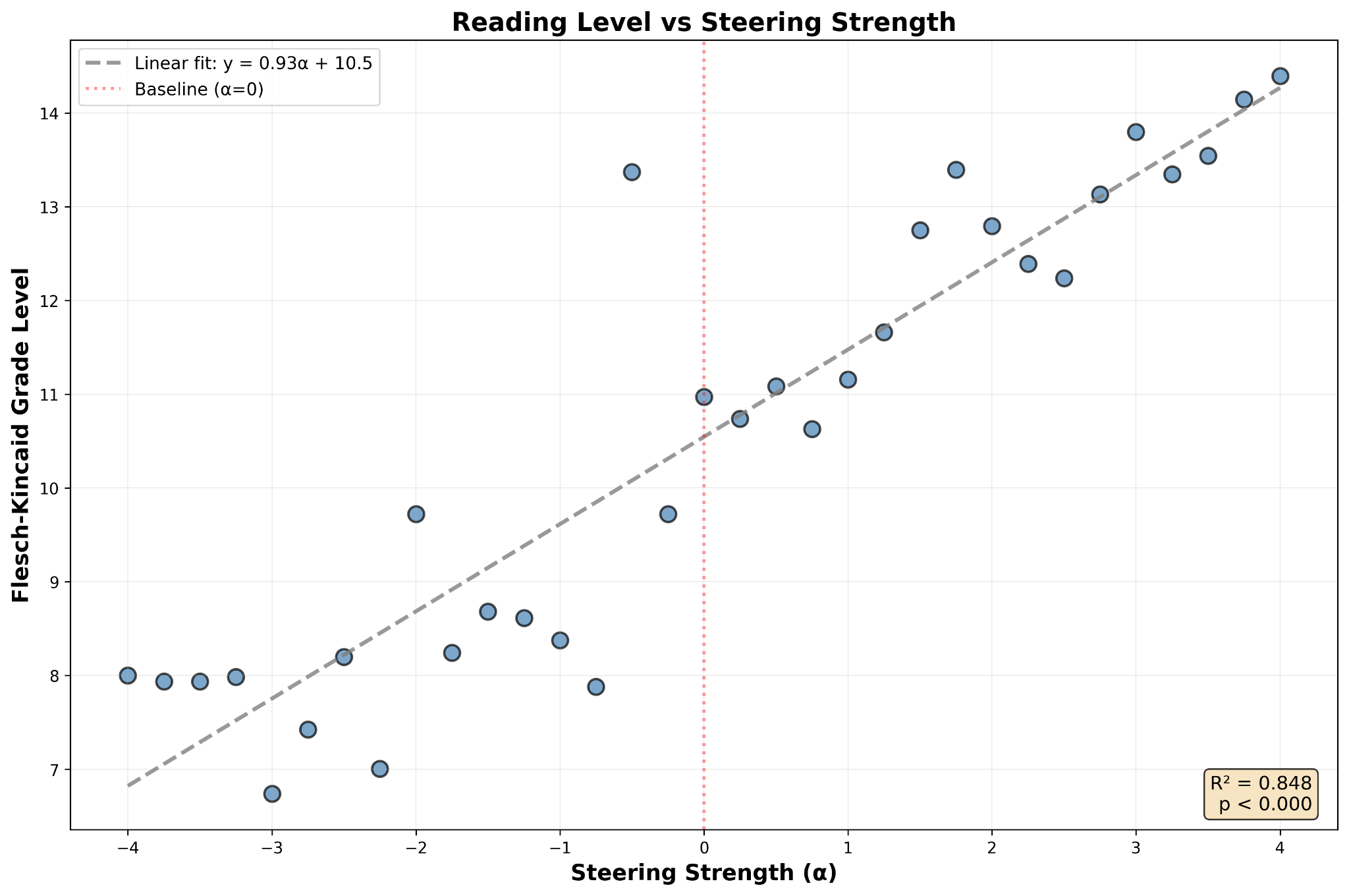
In fact, the results were a conspicuous match for the second experiment’s, with an R² of 0.849, a p-value of 10\^-14 and a slope of 0.931, the numbers we got from Gemma 3 4B IT were sort of within the margin of error of what we saw from Qwen 3 4B Instruct 2507. This once again struck us as improbable.
And The Rest
So we did it all again five more times: Microsoft’s Phi-3 Mini 4K Instruct, Meta’s Llama 3.2 1B Instruct, IBM’s Granite 4.0 Micro, and finally Qwen 3 1.7B and Qwen 3 0.6B, both from Alibaba. With the noteworthy exception of Llama 3.2 1B the results were largely consistent.
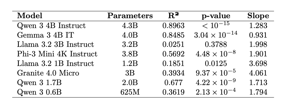
The models were conspicuously consistent in their behavior toward steering along their respective complexity vectors, despite different attention mechanisms, different numbers of layers, and different pre- and post-training methodologies. This is easiest to see when we plot Flesch-Kincaid grade level as a function of steering strength for all eight models on one plot. All the models show a regime of approximate linearity around α = 0 (except for Llama 3.2 3B Instruct) which gives way to extreme nonlinearity the further away one gets from the model’s unsteered state.
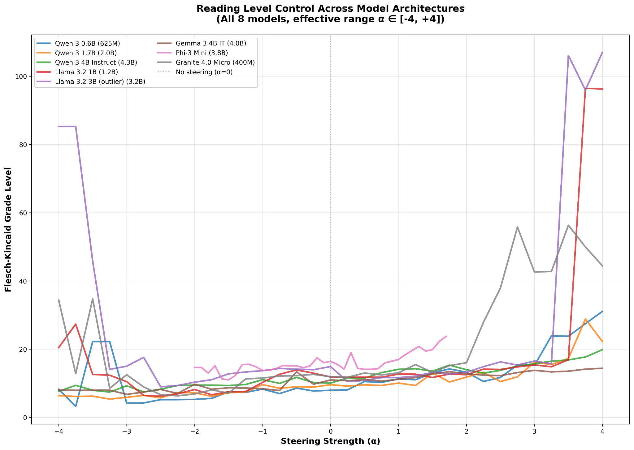
Other interesting observations about this plot include:
-
All the models tested display approximately the same effective range over α, from two or three minus to two or three plus, depending on the model.
-
All the models show similar gains along the complexity vector direction, showing approximately similar slopes in their plots.
-
All the models have an effective range that’s roughly symmetric around α = 0.
Huh. That’s interesting. Symmetric effective ranges…
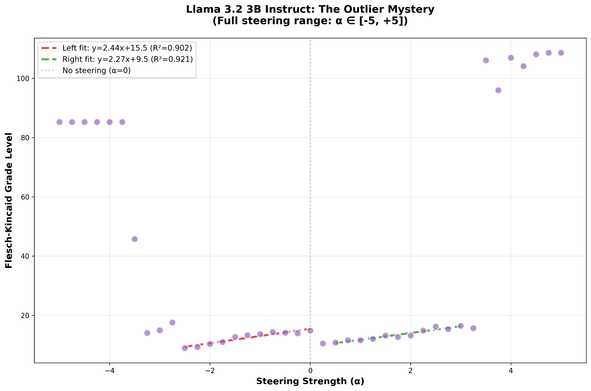
The Mystery of Llama 3.2 3B Instruct
The problem with Llama 3.2 3B Instruct was that we were expect it to respond like Qwen 3 4B Instruct 2507 did: monotonically and symmetrically. In other words, you could swing from -x to x and transition smoothly from one grade level to the next and so on.
Except Llama 3.2 3B Instruct really has two domains of responsiveness to steering that have a discontinuity in the middle.
It’s easier to see if we look more closely.
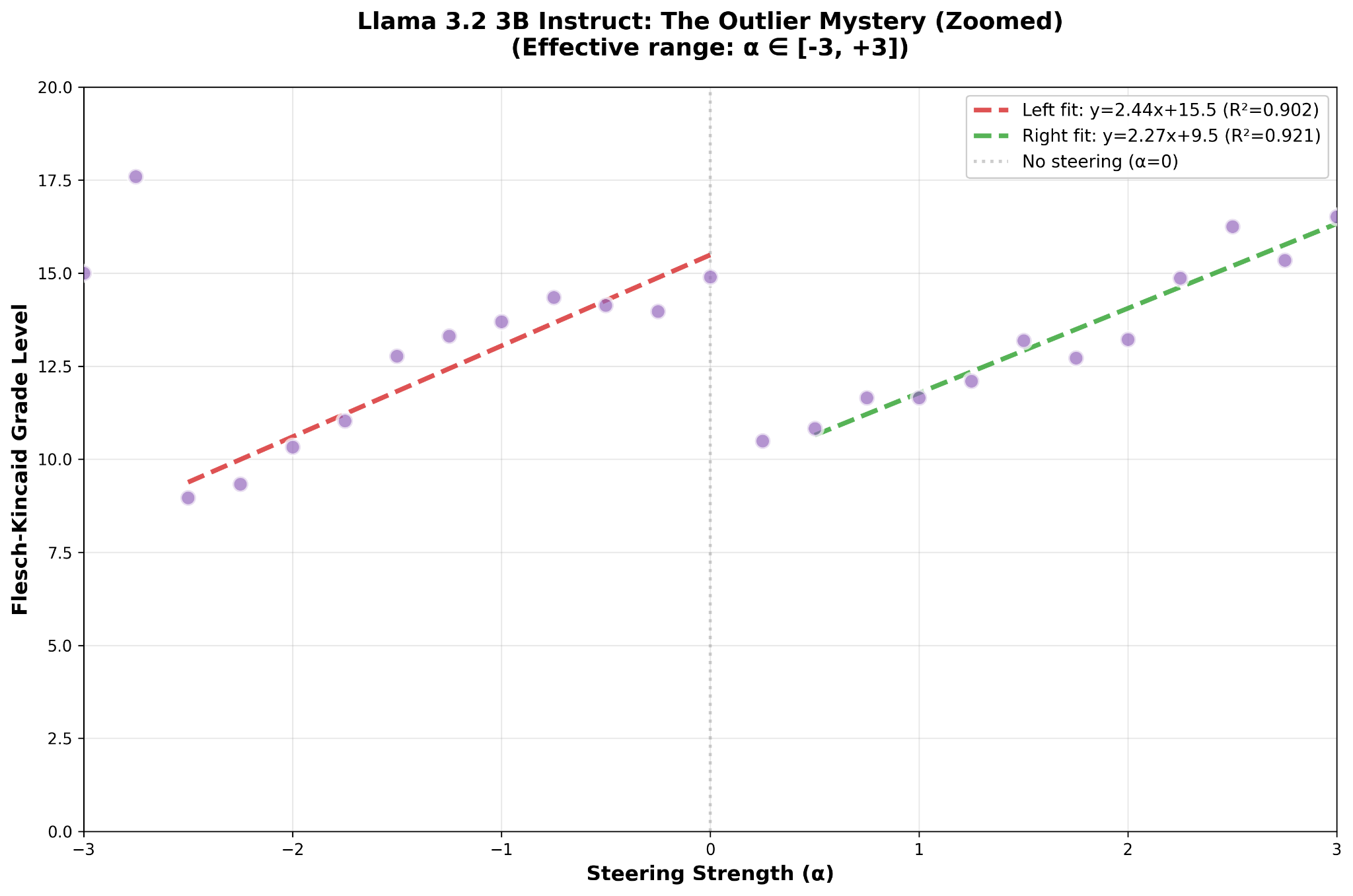
That Llama 3.2 3B Instruct has a piecewise-linear response to steering toward complexity surprised the hell out of us, but in retrospect it really shouldn’t have. Neural networks are, themselves, piecewise-linear functions of several variables. However, that in seven out of eight cases our extracted vector happened to be roughly in the middle of a linear domain while in the case of Llama 3.2 3B Instruct it ended up on the high end of the model’s complexity response curve suggests the possibility that Llama 3.2 3B Instruct is in some way intrinsically different from the other seven tested models.
Conclusions and Questions
We set out to answer the question of whether LLMs could get bored, and ended up with a repeatable method for extracting a steering vector from an LLM which can be used dynamically at inference time to influence output grade level.
We consider this to have been an interesting result.
However, not all our curiosities have been satisfied.
Going Bigger?
For instance, what happens with larger models? Qwen 3 4B Instruct 2507 responded remarkably well to our method. What will the sparse mixture-of-experts model Qwen 3 235B A22B Instruct 2507 do? Will we also find a complexity vector that responds to steering? We will not be finding out right away because that test would require (we estimate) approximately 600 GB of VRAM to run, and the authors are not at this time motivated to rent a whole pod of H100s just to find out.
An alternative would be to use a larger small model such as Qwen 3 32B, although that model could be tricky to work with as it’s a reasoning model that outputs thinking tokens. We’d have to strip those out, or else disable reasoning, so as not to pollute the output and skew the grade level scoring. We could probably rewrite our experimental pipeline to fit a dense 32B model into a single H100, or just run it unmodified on a nice roomy H200.
All this stuff gets in to GPU rental and all that that entails, and so we considered it out-of-scope for the current tinker.
Turn Sampling Back On
The first experiment used sampling — that little bit of randomness at the end of generation that keeps the model from saying the same thing every time you prompt it — with a temperature of 0.7 and a top_p of 0.9. From the second experiment on, we turned sampling off entirely so output was fully deterministic.
An interesting follow-up to this experiment would be to turn sampling back on and run a statistically meaningful number of iterations of each steering experiment. This would show us the variability in output grade level that’s introduced by sampling, if any. For instance, it might be interesting if the variability is very small, within a grade level, versus very large, spanning several grade levels.
That would require running the sampling experiment many, many more times, and we were feeling impatient, so we ruled this question out of scope as well.
The Continuing Mystery of Llama 3.2 3B Instruct
Something is different about Llama 3.2 3B Instruct compared to all the other models. On seven out of eight models, our extraction method resulted in a complexity vector that was more or less in the middle of the steerable range. We could push reading level either up or down by roughly the same magnitude. But with Llama 3.2 3B Instruct, we isolated a complexity vector that’s at the very high range of what the model can produce, and steering with that vector only works if you pull the model away from that maximum.
Then there’s another, equally valid steering domain that covers the range roughly of 0.5 ≤ α ≤ 3.0. Using this domain instead of the first domain gives very similar results in terms of sensitivity and total grade levels spanned; it just happens to be in another part of activation space, across a domain boundary.
If we could find another set of contrasting prompts that isolates a different property of text, we might be able to extract a linear representation that’s close to orthogonal to our complexity vector. The activation space for Qwen 3 4B Instruct 2507 has 2,560 dimensions, so there’s plenty of room to find right-angle vectors.
If we had two orthogonal linear representations, we could steer the model not just along a single axis but along two at the same time, like controlling an Etch-a-Sketch. Given a scalar function of two vectors, we could plot a grid of values over the plan spanning the two extracted vectors in activation space. It would be like radar-mapping terrain. We could pick a point, sample, pick the next point, sample and continue until we have enough points to plot a surface in three dimensions as a function over a tiny sliver of a subspace of activation space.
This might allow us to find and visualize discontinuities in activation space like the one we found in Llama 3.2 3B Instruct.
As this would involve basically starting over from scratch to find another linear representation to extract, we decided it’s kind of a separate thing and that we would tinker with it at a future date.